In this post, I’ll introduce a reinforcement learning (RL) algorithm based on an “alternative” paradigm: divide and conquer. Unlike traditional methods, this algorithm is not based on temporal difference (TD) learning (which has scalability challenges), and scales well to long-horizon tasks.
We can do Reinforcement Learning (RL) based on divide and conquer, instead of temporal difference (TD) learning.
Problem setting: off-policy RL
Our problem setting is off-policy RL. Let’s briefly review what this means.
There are two classes of algorithms in RL: on-policy RL and off-policy RL. On-policy RL means we can only use fresh data collected by the current policy. In other words, we have to throw away old data each time we update the policy. Algorithms like PPO and GRPO (and policy gradient methods in general) belong to this category.
Off-policy RL means we don’t have this restriction: we can use any kind of data, including old experience, human demonstrations, Internet data, and so on. So off-policy RL is more general and flexible than on-policy RL (and of course harder!). Q-learning is the most well-known off-policy RL algorithm. In domains where data collection is expensive (e.g., robotics, dialogue systems, healthcare, etc.), we often have no choice but to use off-policy RL. That’s why it’s such an important problem.
As of 2025, I think we have reasonably good recipes for scaling up on-policy RL (e.g., PPO, GRPO, and their variants). However, we still haven’t found a “scalable” off-policy RL algorithm that scales well to complex, long-horizon tasks. Let me briefly explain why.
Two paradigms in value learning: Temporal Difference (TD) and Monte Carlo (MC)
In off-policy RL, we typically train a value function using temporal difference (TD) learning (i.e., Q-learning), with the following Bellman update rule:
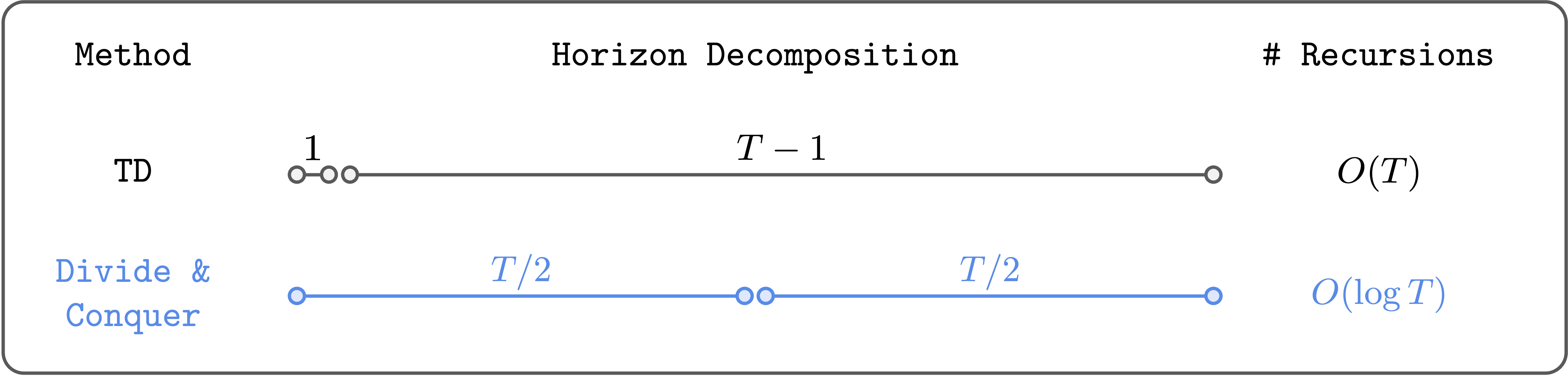
\[\begin{aligned} Q(s, a) \gets r + \gamma \max_{a'} Q(s', a'), \end{aligned}\]The problem is this: the error in the next value $Q(s’, a’)$ propagates to the current value $Q(s, a)$ through bootstrapping, and these errors accumulate over the entire horizon. This is basically what makes TD learning struggle to scale to long-horizon tasks (see this post if you’re interested in more details).
To mitigate this problem, people have mixed TD learning with Monte Carlo (MC) returns. For example, we can do $n$-step TD learning (TD-$n$):
\[\begin{aligned} Q(s_t, a_t) \gets \sum_{i=0}^{n-1} \gamma^i r_{t+i} + \gamma^n \max_{a'} Q(s_{t+n}, a'). \end{aligned}\]Here, we use the actual Monte Carlo return (from the dataset) for the first $n$ steps, and then use the bootstrapped value for the rest of the horizon. This way, we can reduce the number of Bellman recursions by $n$ times, so errors accumulate less. In the extreme case of $n = \infty$, we recover pure Monte Carlo value learning.
While this is a reasonable solution (and often works well), it is highly unsatisfactory. First, it doesn’t fundamentally solve the error accumulation problem; it only reduces the number of Bellman recursions by a constant factor ($n$). Second, as $n$ grows, we suffer from high variance and suboptimality. So we can’t just set $n$ to a large value, and need to carefully tune it for each task.
Is there a fundamentally different way to solve this problem?
The “Third” Paradigm: Divide and Conquer
My claim is that a third paradigm in value learning, divide and conquer, may provide an ideal solution to off-policy RL that scales to arbitrarily long-horizon tasks.
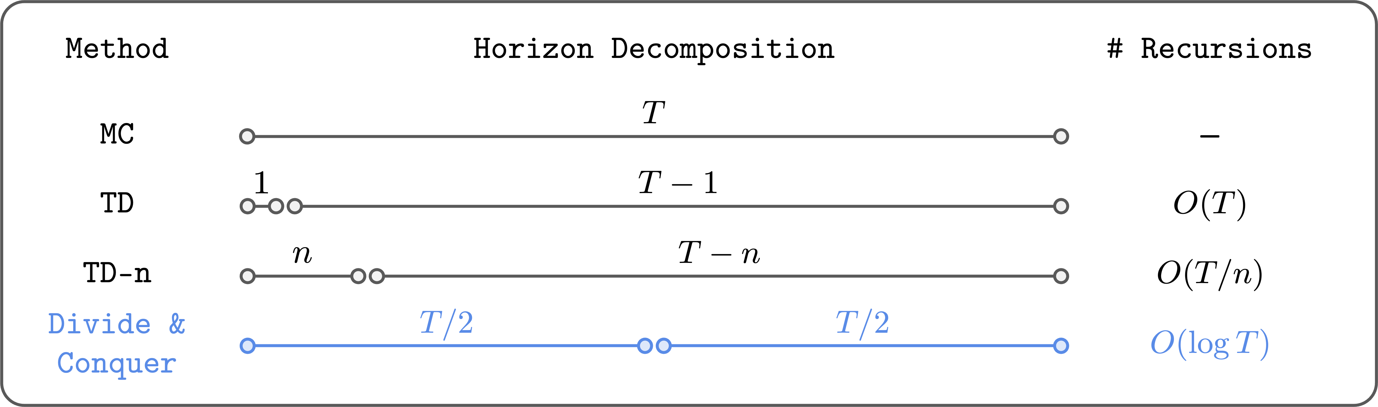
Divide and conquer reduces the number of Bellman recursions logarithmically.
The key idea of divide and conquer is to divide a trajectory into two equal-length segments, and combine their values to update the value of the full trajectory. This way, we can (in theory) reduce the number of Bellman recursions logarithmically (not linearly!). Moreover, it doesn’t require choosing a hyperparameter like $n$, and it doesn’t necessarily suffer from high variance or suboptimality, unlike $n$-step TD learning.
Conceptually, divide and conquer really has all the nice properties we want in value learning. So I’ve long been excited about this high-level idea. The problem was that it wasn’t clear how to actually do this in practice… until recently.
A practical algorithm
In a recent work co-led with Aditya, we made meaningful progress toward realizing and scaling up this idea. Specifically, we were able to scale up divide-and-conquer value learning to highly complex tasks (as far as I know, this is the first such work!) at least in one important class of RL problems, goal-conditioned RL. Goal-conditioned RL aims to learn a policy that can reach any state from any other state. This provides a natural divide-and-conquer structure. Let me explain this.
The structure is as follows. Let’s first assume that the dynamics is deterministic, and denote the shortest path distance (“temporal distance”) between two states $s$ and $g$ as $d^*(s, g)$. Then, it satisfies the triangle inequality:
\[\begin{aligned} d^*(s, g) \leq d^*(s, w) + d^*(w, g) \end{aligned}\]for all $s, g, w \in \mathcal{S}$.
In terms of values, we can equivalently translate this triangle inequality to the following “transitive” Bellman update rule:
\[\begin{aligned} V(s, g) \gets \begin{cases}\gamma^0 & \text{if } s = g, \\\\ \gamma^1 & \text{if } (s, g) \in \mathcal{E}, \\\\ \max_{w \in \mathcal{S}} V(s, w)V(w, g) & \text{otherwise}\end{cases} \end{aligned}\]where $\mathcal{E}$ is the set of edges in the environment’s transition graph, and $V$ is the value function associated with the sparse reward $r(s, g) = 1(s = g)$. Intuitively, this means that we can update the value of $V(s, g)$ using two “smaller” values: $V(s, w)$ and $V(w, g)$, provided that $w$ is the optimal “midpoint” (subgoal) on the shortest path. This is exactly the divide-and-conquer value update rule that we were looking for!
The problem
However, there’s one problem here. The issue is that it’s unclear how to choose the optimal subgoal $w$ in practice. In tabular settings, we can simply enumerate all states to find the optimal $w$ (this is essentially the Floyd-Warshall shortest path algorithm). But in continuous environments with large state spaces, we can’t do this. Basically, this is why previous works have struggled to scale up divide-and-conquer value learning, even though this idea has been around for decades (in fact, it dates back to the very first work in goal-conditioned RL by Kaelbling (1993) – see our paper for a further discussion of related works). The main contribution of our work is a practical solution to this issue.
The solution
Here’s our key idea: we restrict the search space of $w$ to the states that appear in the dataset, specifically, those that lie between $s$ and $g$ in the dataset trajectory. Also, instead of searching for the optimal $\text{argmax}_w$, we compute a “soft” $\text{argmax}$ using expectile regression. Namely, we minimize the following loss:
\[\begin{aligned} \mathbb{E}\left[\ell^2_\kappa (V(s_i, s_j) - \bar{V}(s_i, s_k) \bar{V}(s_k, s_j))\right], \end{aligned}\]where $\bar{V}$ is the target value network, $\ell^2_\kappa$ is the expectile loss with an expectile $\kappa$, and the expectation is taken over all $(s_i, s_k, s_j)$ tuples with $i \leq k \leq j$ in a randomly sampled dataset trajectory.
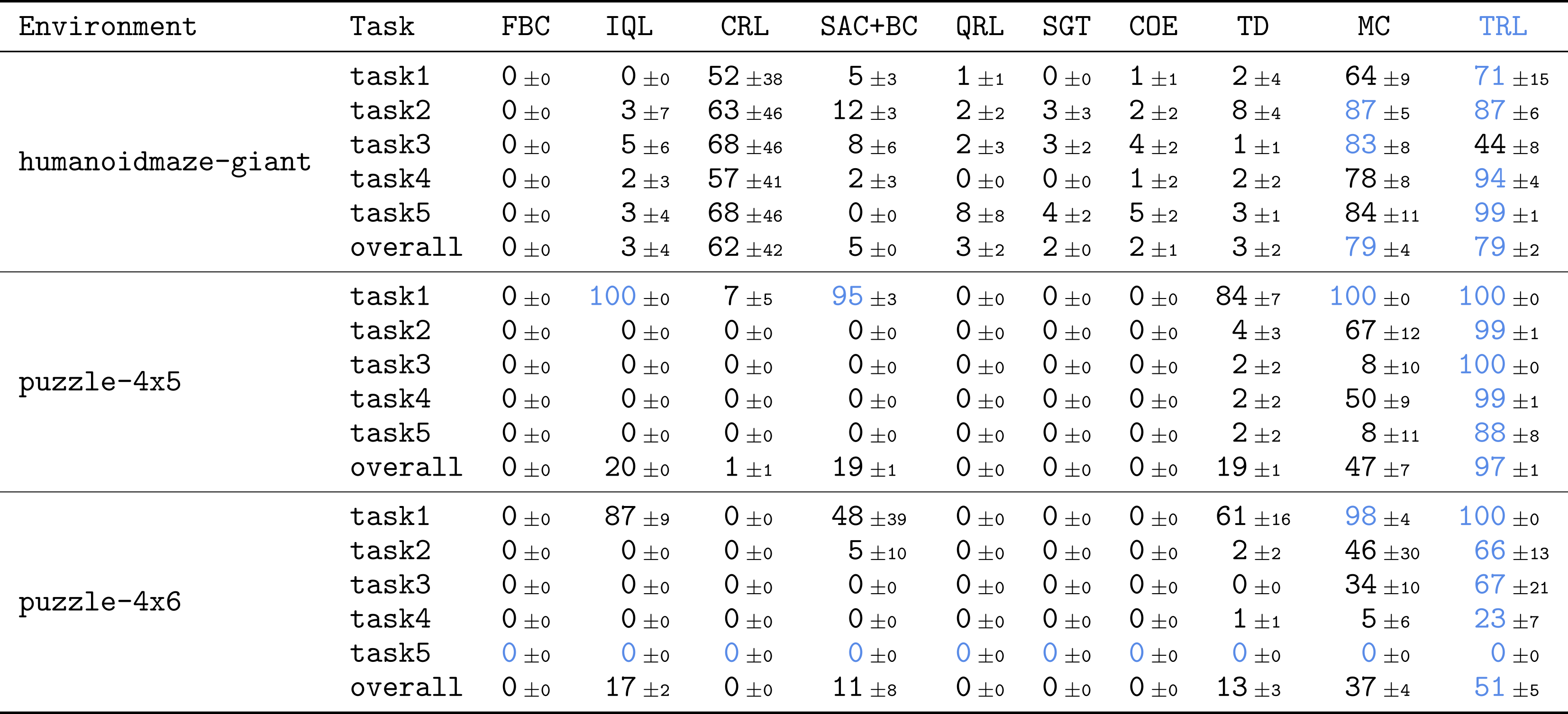
This has two benefits. First, we don’t need to search over the entire state space. Second, we prevent value overestimation from the $\max$ operator by instead using the “softer” expectile regression. We call this algorithm Transitive RL (TRL). Check out our paper for more details and further discussions!
Does it work well?
humanoidmaze