💡 **类比ML训练设计电子元件：** 文章的核心在于将机器学习中的训练过程应用于电子元件设计。通过设定输入、中间和输出三个接口（API），并明确每个接口的电压范围，来约束串联的两个电子元件的行为，使其整体功能类似于数字身份函数，即保持逻辑值的准确传递，同时对电压进行缓冲和净化。

🔗 **接口（APIs）与约束：** API是连接电子元件的关键。每个API定义了逻辑0和逻辑1对应的电压范围。元件1的输出必须符合API2的约束，元件2的输出必须符合API3的约束。这种接口定义为组件的设计提供了明确的输入和输出规范，确保了系统的整体行为符合预期，并为解耦训练奠定了基础。

🧩 **解耦训练与熵最大化：** 这种方法的一个重要优势在于组件的解耦。每个元件的参数选择只需要满足其相邻的API约束，而与其他元件的内部工作机制无关。结合统计力学的思想，作者推测训练过程会倾向于寻找能够实现这些接口约束且拥有最大可能参数组合（即最大化熵）的API集合，这有助于提升设计的鲁棒性和灵活性。

🚀 **提升系统鲁棒性与可解释性：** 通过类比ML训练和引入接口概念，该模型不仅能设计出能够接受不精确输入并提供更精确输出的电子元件，从而提高系统的鲁棒性和可扩展性，还能为理解机器学习模型内部结构和工作机制提供新的思路，弥合了统计力学理论与模型可解释性之间的差距。

Published on November 6, 2025 11:21 PM GMT

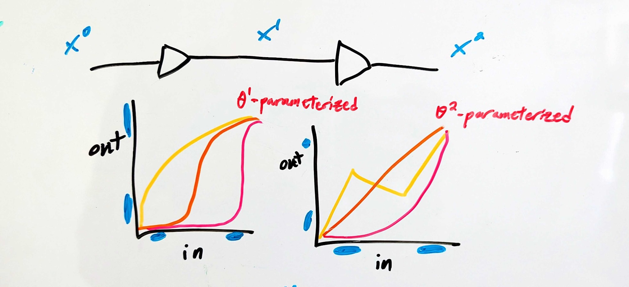
Imagine using an ML-like training process to design two simple electronic components, in series. The parameters ${\theta }^{}$ control the function performed by the first component, and the parameters ${\theta }^{}$ control the function performed by the second component. The whole thing is trained so that the end-to-end behavior is that of a digital identity function: voltages close to logical 1 are sent close to logical 1, voltages close to logical 0 are sent close to logical 0.

Background: Signal Buffering

We’re imagining electronic components here because, for those with some electronics background, I want to summon to mind something like this:

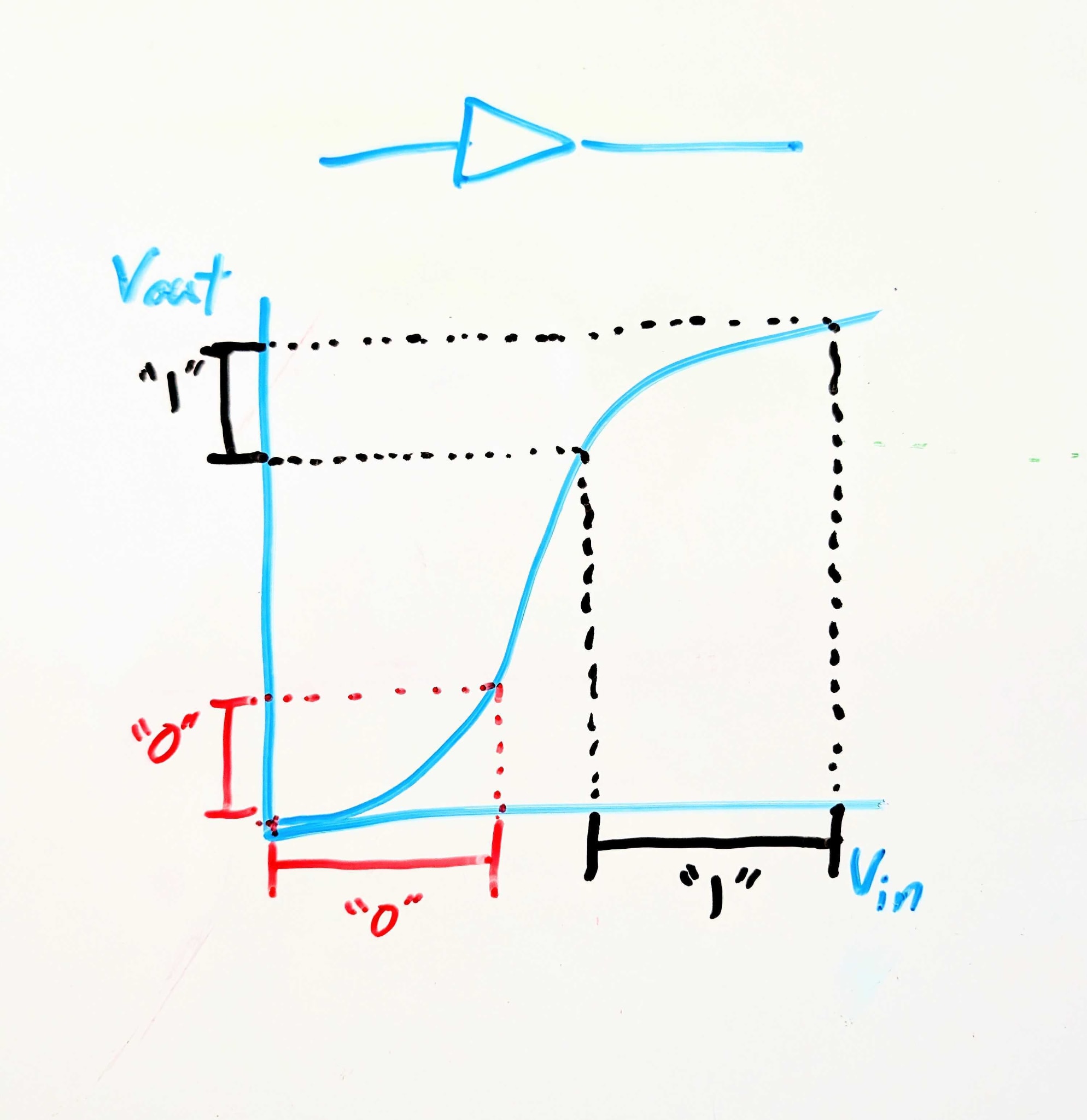
This electronic component is called a signal buffer. Logically, it’s an identity function: it maps 0 to 0 and 1 to 1. But crucially, it maps a wider range of logical-0 voltages to a narrower (and lower) range of logical-0 voltages, and correspondingly for logical-1. So if noise in the circuit upstream might make a logical-1 voltage a little too low or a logical-0 voltage a little too high, the buffer cleans that up, pushing the voltages closer to their ideal values.

This is a generalizable point about interfaces in scalable systems: for robustness and scalability, components need to accept less-precise inputs and give more-precise outputs.

That’s the background mental picture I want to invoke. But now, I want to combine it with an ML-like mental picture of training a system to match particular input/output behavior.

Back To The Original Picture: Introducing Interfaces

Here’s a conceptual story.

There are three interfaces - “APIs”, we’ll call them. The first ($AP{I}^{}$) is at the input of the whole system, the second ($AP{I}^{}$) between the two components, and the last ($AP{I}^{}$) is at the output of the whole system. At each of those APIs, there’s a set of “acceptable” voltages for each logical input to the full system (i.e. 0 or 1).

The APIs constrain the behavior of each component - e.g. component 1 is constrained by $AP{I}^{}$ (which specifies its inputs) and $AP{I}^{}$ (which specifies its outputs).

Let's put some math on that, with some examples.

A set of APIs might look like:

$AP{I}^{}:(0\mapsto [0V,1.2V],1\mapsto [3.5V,5.0V\left]\right)$ - i.e. the full system accepts either a voltage between 0 and 1.2 volts (representing logical 0), or a voltage between 3.5 and 5.0 volts (representing logical 1). No particular behavior is guaranteed for other voltages.$AP{I}^{}:(0\mapsto [0V,0.5V]\cup [4.6V,5.0V],1\mapsto [2.6V,3.8V\left]\right)$ - i.e. in the middle the system uses extreme voltages (either above 4.6 or below 0.5 volts) to represent logical 0, and middling voltages to represent logical 1. Weird, but allowed.$AP{I}^{}:(0\mapsto [0V,0.5V],1\mapsto [2.8V,5.0V\left]\right)$ - i.e. a narrower range of low voltages but wider range of high voltages, compared to the input. This might not be the most useful circuit behavior, but it’s an allowed circuit behavior.

(For simplicity, we’ll assume all voltages are between 0V and 5V). In order for the system to satisfy those particular APIs:

Component 1 must map every value in $AP{I}^{}\left(0\right)$ to a value in $AP{I}^{}\left(0\right)$, and every value in $AP{I}^{}\left(1\right)$ to a value in $AP{I}^{}\left(1\right)$ - i.e. any value less than 1.2V must be mapped either below 0.5V or above 4.6V, while any value above 3.5V must be mapped between 2.6 and 3.8V.Component 2 must likewise map every value in $AP{I}^{}\left(0\right)$ to a value in $AP{I}^{}\left(0\right)$, and every value in $AP{I}^{}\left(1\right)$ to a value in $AP{I}^{}\left(1\right)$.

Using $f^{}i$ for component $i$ and writing it out mathematically: the components satisfy a set of APIs if and only if

$\forall b\in 0,1,x\in AP{I}^{}\left(b\right):f^{}i$(x,θi)∈APIi+1(b)

That’s a set of constraints on ${\theta }^{}$, for each component $i$.

The Stat Mech Part

So the APIs put constraints on the components. Furthermore, subject to those constraints, the different components decouple: component 1 can use any parameters ${\theta }^{}$ internally so long as it satisfies the API set (specifically $AP{I}^{}$ and $AP{I}^{}$), and component 2 can use any parameters ${\theta }^{}$ internally so long as it satisfied the API set (specifically $AP{I}^{}$ and $AP{I}^{}$).

Last big piece: putting on our stat mech/singular learning theory hats, we educatedly-guess that the training process will probably end up with an API set which can be realized by many different parameter-values. A near-maximal number of parameter values, probably.

The decoupling now becomes very handy. Let’s use the notation $H(\Theta |<constraints>)$ - you can think of it as the log number of parameter values compatible with the constraints, or as entropy or relative entropy of parameters given constraints (if we want to weight parameter values by some prior distribution, rather than uniformly). Because of the decoupling, we can write H as

$H\left(\Theta |API\right)=$

$H({\Theta }^{}|\forall b\in 0,1,x\in AP{I}^{}$(x,θ1)∈API2(b))

$+H({\Theta }^{}|\forall b\in 0,1,x\in AP{I}^{}$(x,θ2)∈API3(b))

So there’s one term which depends only on component 1 and the two APIs adjacent to component 1, and another term which depends only on component 2 and the two APIs adjacent to component 2.

Our stat-mech-ish prediction is then that the training process will end up with a set of APIs for which $H\left(\Theta |API\right)$ is (approximately) maximal.

Why Is This Interesting?

What we like about this mental model is that it bridges the gap between stat mech/singular learning theory flavored intuitions (i.e. training finds structure compatible with the most parameters, subject to constraints) and internal structures in the net (i.e. internal interfaces). This feels to us like exactly the gap which needs to be crossed in order for stat mech flavored tools to start saying big things about interpretability.