本研究深入探讨了大语言模型（LLMs）中一种名为“激活平台”的非线性现象。通过分析模型在不同输入序列间的插值过程，研究发现激活平台并非模型架构固有，而是模型学习所得，且与模型处理信息的方式密切相关。文章详细阐述了激活平台如何随着模型层数的加深而逐渐形成和锐化，并指出多层感知机（MLP）在其中扮演了关键角色。此外，研究还发现激活平台的存在与否与LayerNorm层无关，且平台边界与MLP的输入-输出敏感度区域高度吻合。这些发现不仅为理解LLMs的内部机制提供了新视角，也将其与模型梯度、决策边界等其他研究领域建立了联系。

💡 **激活平台是模型学习的非线性现象**：研究表明，大语言模型（LLMs）在处理不同输入序列时，激活值变化并非线性，而是可能出现“激活平台”——即在大部分插值过程中变化微小，随后发生剧烈“相变”。这种现象并非模型架构预设，而是模型在训练过程中学习到的，是理解模型信息转换机制的关键。

🚀 **MLP是激活平台形成的核心驱动力**：实验结果明确指出，多层感知机（MLP）在激活平台的形成中起着决定性作用。通过冻结模型不同组件的输出，研究发现，MLP的输出变化是激活平台产生和变化的必要条件，而注意力机制（Attention）在此过程中影响甚微。这表明MLP是模型进行复杂信息转换和特征提取的关键。

📈 **激活平台与MLP敏感度区域相关**：文章进一步揭示，激活平台中的“平台边界”（即剧烈变化区域）与MLP的输入-输出敏感度高度相关。研究通过计算MLP的雅可比矩阵范数发现，在平台边界处，MLP的敏感度会急剧升高。这表明模型在这些区域会放大输入的变化，从而导致输出的快速转变，这可能与模型识别和区分不同语义类别有关。

🔗 **激活平台与多项研究领域相连**：激活平台的研究与模型梯度、决策边界、以及神经网络的泛化能力等多个前沿研究领域存在深刻联系。例如，平台边界的形成机制可能与模型在决策边界附近的“放大”效应类似，并且与模型在训练数据流形上的低敏感度区域有关，为理解模型的泛化能力和鲁棒性提供了新的视角。

Published on October 17, 2025 5:48 AM GMT

By design, LLMs perform nonlinear mappings from their inputs (text sequences) to their outputs (next-token generations). Some of these nonlinearities are built-in to the model architecture, but others are learned by the model, and may be important parts of how the model represents and transforms information. By studying different aspects of this nonlinear mapping, we can aim to understand how these models make sense of their inputs and respond to them.

An example of such learned nonlinearities is that of activation plateaus—a phenomenon where interpolating from one input sequence to another can produce minimal downstream changes for most of the interpolation, with a sudden rapid 'phase change' somewhere in the middle. This raises interesting questions about the nature of continuous feature representations (e.g. the Linear Representation Hypothesis), and has potential implications for various interpretability methods, such as model steering. Furthermore, if plateaus are strongly related to model features, then they may afford new methods for uncovering these features.

In this post, we provide a general mechanistic explanation of where—and to some degree how—activation plateaus emerge. These findings connect the activation plateau phenomenon to other active research areas and provide concrete directions for future projects.

This work was done as part of a PIBBSS Summer Research Fellowship (2025).

Full code for all experiments can be found at https://github.com/MShinkle/activation_plateau_mechanisms.

Brief Background on Activation Plateaus

The basic method for eliciting activation plateaus is moderately simple. Start by taking two text sequences which are completely identical except for the last token. For example:

"The house was big""The house was in"

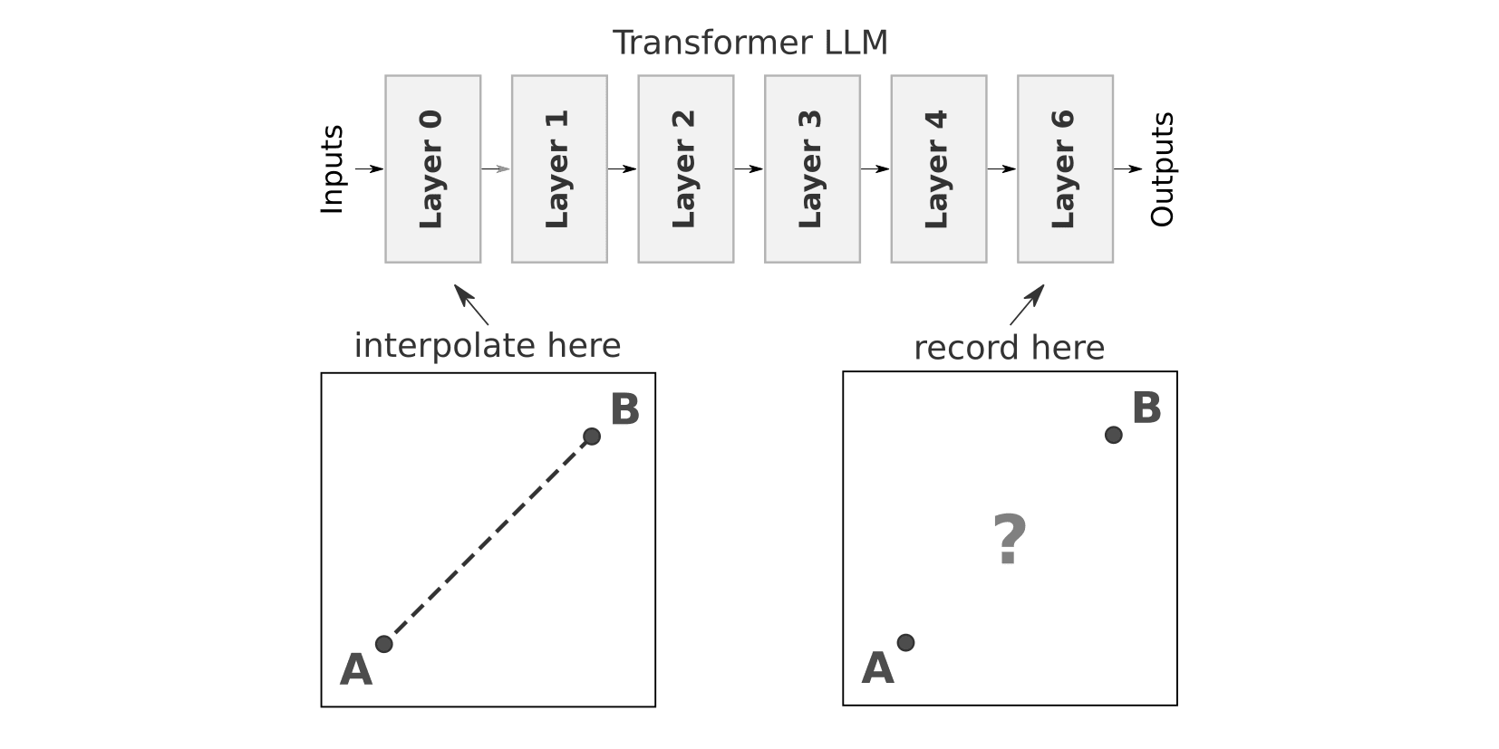
Take these two sequences, pass them into a transformer-based LLM, and collect the activations somewhere early in the model, e.g. the embeddings or outputs of the first layer. These should be identical for all tokens except the last one. 

Next, smoothly interpolate the recorded activations for the two sequences at the last token. This can be linear interpolation or (as we use in the experiments in this post) spherical interpolation^[1].

For each interpolation step, patch the interpolated activations back into the model, and record the resulting model outputs (logits). Finally, compute the relative (L2) distance of the outputs for each interpolation step to the original outputs for the two sequences.^[2]

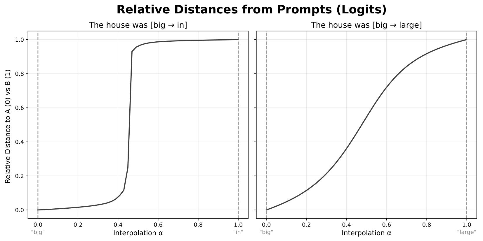
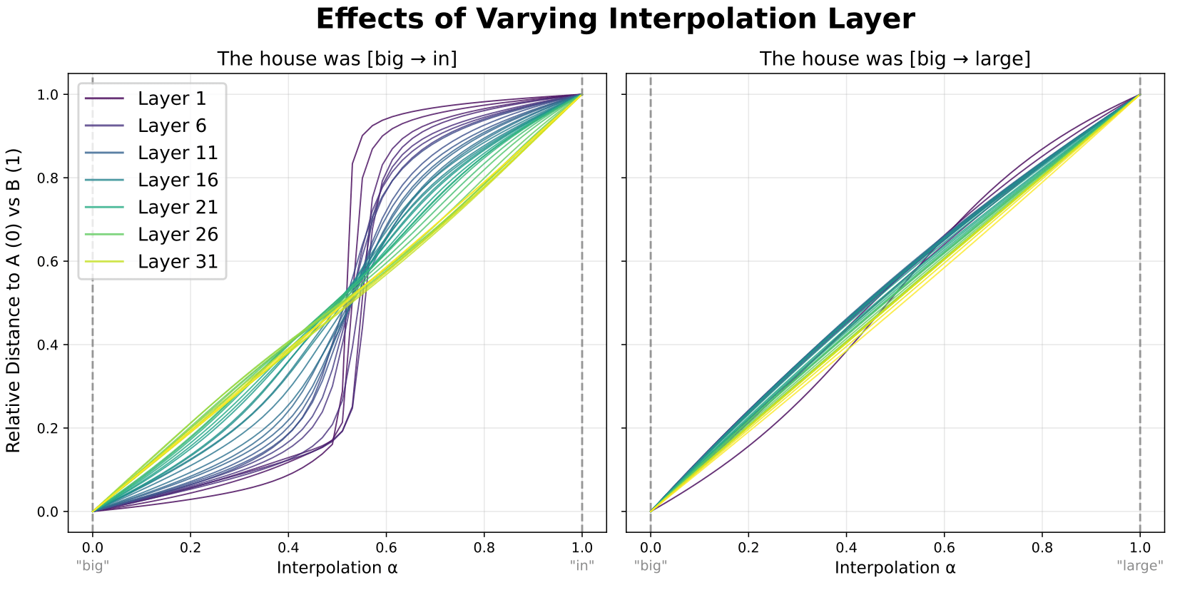
If we plot these relative distances, we see a couple different types of curves. Sometimes, like the rightmost plot below, the curves are fairly straight, suggesting that changes early in the model result in fairly constant changes in the model outputs. But in other cases, like the plot below on the left, interpolating toward sequence B has little effect on the outputs at first, then produces a sudden, rapid change where outputs go from being similar to those for sequence A to those for sequence B. Outputs then remain relatively unchanged for the rest of the interpolation.

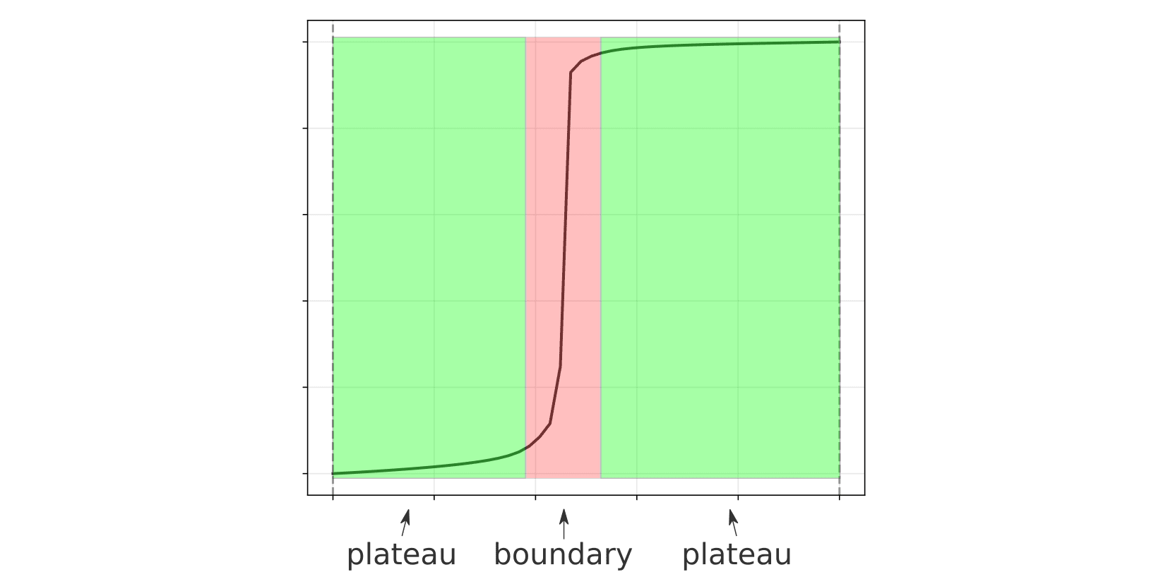
These areas of low change are what we refer to as 'plateaus', and the area of sharp change between them are plateau 'boundaries'.

So where—and how—do plateaus and boundaries actually emerge within LLMs? In the following experiments, we systematically examine how different layers and model components shape plateaus and boundaries. We also provide a general, but useful, mechanistic explanation for how they arise.

All experiments are done using a trained GPT-2 Large model. We show examples for both plateau (left) and non-plateau (right) prompt pairs, but focus primarily on the plateau case. Unless otherwise noted, we interpolate and record at layer outputs, using the resid_post hook in TransformerLens.

Experimental Results

Plateaus Emerge Gradually Across Layers

We first looked at how plateaus vary across model layers. Instead of just recording and plotting model logits, we instead recorded activations in each layer downstream of the interpolation, and plotted the relative distance curves for each.

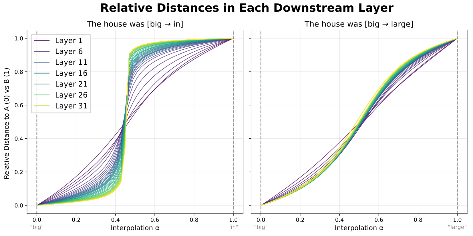
As shown in the figure above, plateaus emerge gradually across model layers, with each successive layer flattening out the plateaus and sharpening the boundary between them.

Another complementary way to do this is rather than varying they layer we record at, we vary the layer we interpolate at. Specifically, we always record the outputs of the last model layer (layer 35), and vary the layer at which the activations are interpolated and patched into the model.

This shows a complementary result—the earlier in the model we interpolate, the flatter the plateaus and the sharper the boundary. This suggests that the principal factor here is is the number of layers between interpolation and recording.

We can test this specific hypothesis directly by varying both the interpolation layer (L) and recording layer (L+N) while keeping the number of layers between them (N) fixed.

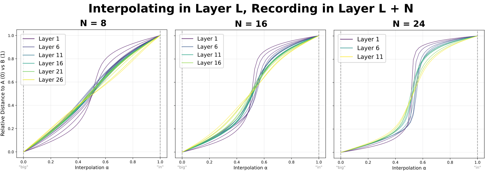
Indeed, increasing the number of layers (N) between interpolation and recording increases the sharpness of the plateaus. With that said, this plot does also show an effect of depth (L) in the model: earlier layers sharpen plateaus relatively more than do later layers. But the fact that plateaus still emerge when interpolation is done late in the model suggest that all layers are having a similar type of effect, just varying in strength.

Taken together, these results show that activation plateaus emerge and sharpen gradually across model layers, with later layers having a slightly weaker—but similar—effect.

Plateaus Emerge From MLPs

We want to know whether these plateaus are created by the attention- or MLP blocks in our model. To isolate these effects we repeated the interpolation experiment while freezing the output of the attention- or MLP layer.

 Specifically, at each layer, we set the output activations (attn_out or mlp_out) to the average activations across all interpolation steps. By freezing the outputs of the attention or MLP blocks to be the same for all interpolation steps, variation in model outputs must be due to variation in the output of the other, non-frozen component.

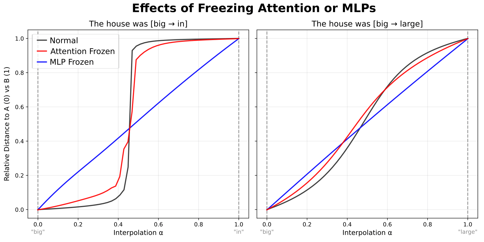
When resulting relative distances are plotted as above, we find that freezing the outputs of the attention blocks has relatively small effects on the resulting curves (red lines). Therefore, variation in attention block outputs is not necessary for plateaus to emerge. In contrast, freezing of MLP block outputs completely eliminates the plateaus (blue lines). Together, these results tie plateaus specifically to MLP blocks, showing that variation in MLP outputs is necessary—and is largely sufficient—to account for how plateaus emerge. 

Plateaus Emerge Without Layernorm

In GPT-2-style transformers, MLP blocks can be broken down into an initial LayerNorm operation, which rescales and shifts the data, and the actual MLP component, which consists of two fully-connected (FC) layers and a nonlinearity. The LayerNorm operation is notoriously annoying for a variety of mechanistic interpretability methods. Is it necessary for plateaus to occur?

To test this, we used the LayerNorm-free variant of  GPT-2 Large from Baroni et al. (a fine-tuned of GPT-2 Large that replaces LayerNorm with a linear operation).

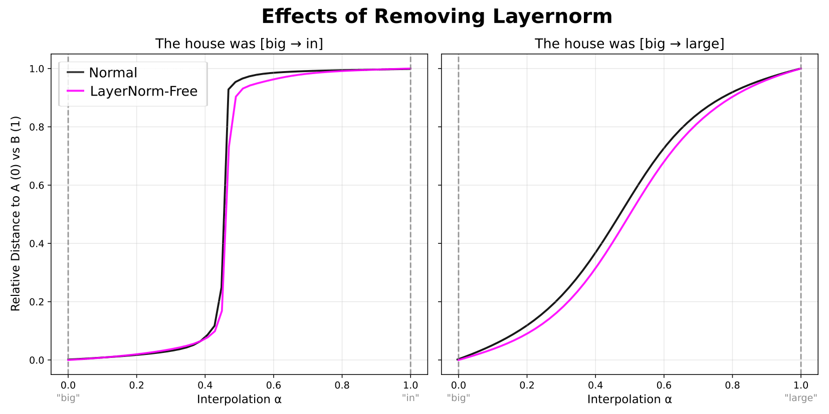
As shown above, when we perform the basic activation plateau experiment again with this LayerNorm-free variant, we get almost identical relative distance curves as with the regular model.^[3] While this does not definitively rule out any involvement in producing plateaus, this shows that either a) LayerNorm isn't involved in producing activation plateaus, or b) that whatever role LayerNorm does plays can learned by other parts of the model instead.^[4] Examining plateaus in LayerNorm-free models should enable a wider range of techniques to be applied to the MLPs in order to better understand plateaus.

Plateaus and Boundaries Correspond to Areas of Low and High MLP Sensitivity

Given our findings thus far, we should be able to tie plateaus and their boundaries specifically to properties of the MLPs themselves. As an exploration of this, we examined whether plateaus and boundaries can be explained by areas of low and high input-output sensitivity in the layerwise MLPs.

First, we measured the step sizes—the differences (L2) between downstream activations for subsequent interpolation steps.

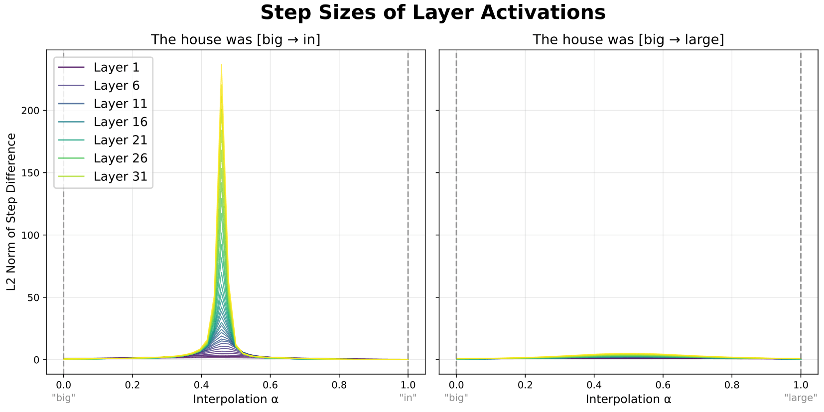
When plotted, we see that plateau boundaries correspond to areas where step sizes suddenly peak. This is expected; after all, plateau boundaries are defined as areas of rapid change in the relative similarities to the two reference prompts^[5]

Next, we computed Jacobians of the activations (not the weights), mapping to MLP outputs for a given set of MLP inputs. We did this for each interpolation step, and computed the L2 (Frobenius) norms of these stepwise Jacobians as an aggregate metric of the input-output sensitivity.^[6]

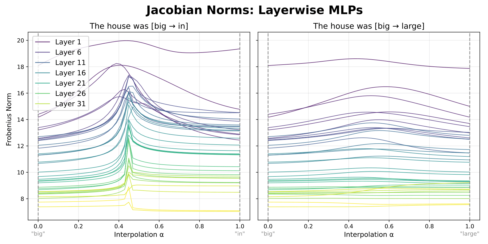
As shown above, we see a clear spike in the magnitudes of the activation Jacobians in the same area where step sizes also peak. Furthermore, while these spikes are wider for early layers, they increase in sharpness as we look at layers deeper in the model.^[7]

This all ties together in the following picture:

MLP Jacobians are consistently (across layers) higher in magnitude somewhere along the interpolation path between the two prompts.^[8]These Jacobians accumulate (roughly) multiplicatively across layers, resulting in sharper and larger-magnitude peaks as you look at deeper layers.Because the Jacobians determine the amount of change in MLP outputs as a function of MLP inputs, inputs that fall in low-Jacobian areas tend to map to very similar outputs, resulting in plateaus. Only points that fall in the area where the Jacobians spike end up mapped to substantially diverging outputs.Indeed, if we measure the relative distance to the two endpoints (prompts) at each step, we get a very similar curve to the plateaus observed in real models.

While there are indubitably nuances that this picture doesn't capture, it effectively ties together our findings: that activation plateaus emerge and sharpen gradually across layers; the their formation can be tied specifically to layer MLPs, and that plateaus and boundaries correspond to areas of low and high input-output sensitivity in the MLPs.

Connections to Other Research Areas

One exciting thing about these findings is that they link the phenomenon of activation plateaus to other phenomena and research areas.

Jacobian-Based Sensitivity

For example, other research projects have examined the effects of steering models along high- versus low-sensitivity directions, based on the model input-output Jacobians. Examples of such works include:

Unveiling Transformer Perception by Exploring Input Manifolds (Benfenati et al.,  2024) The authors use activation Jacobians to find paths along the input space which yield the same or similar model outputs. While they primarily focus on vision models and BERT, these or similar methods may be used to characterize the shapes and locations of plateaus in model activation space.

Neural networks learn to magnify areas near decision boundaries (Zavatone-Veth et al., 2023). The authors find that classification models tend to 'magnify' areas of activation space  around learned decision boundaries (measured via a volume metric of activation Jacobians). Given that we also find a sort of Jacobian-based 'magnification' around plateau boundaries, this suggests that plateau boundaries may correspond to distinct, but related semantic categories.

Sensitivity and Generalization in Neural Networks: an Empirical Study (Novak et al., 2018). The authors use Jacobian-based measures of input sensitivity to characterize the effects of input perturbations, finding that the training data manifold corresponds to areas of low sensitivity (and therefore high perturbation robustness). This raises the possibility that plateau boundaries, where Jacobian norms are high, might correspond to points moving off of the training data manifold.

Relationships Between Loss Landscapes and Activation Spaces. Learning theories (various) and SLT (Watanabe et al., 2013, Murfet et al., 2020) have shown that models which lie in wide, flat regions of the loss landscape tend to generalize better than models in areas of higher curvature. While this landscape lies in the space of model parameters, does this have implications for activation space? If so, could this explain why real activations tend to lie within broad, low-Jacobian plateaus? If you have ideas or papers relating to this, we would be very curious to hear about them.

MLP Splines and Polytopes

Another research area our results connect to activation plateaus is that of MLP 'splines'. In the case of models using ReLU as their activation function, these splines can be defined as the 'decision boundary' for an individual neuron, where its activation goes from being less than the ReLU threshold (thus outputting 0) to being above the threshold (thus outputting >0). Previous works in classification models (Humayun et al. 2023, 2024) have shown that GELU splines tend to tightly organize themselves along learned classifications boundaries. 

If it is true that both 1) plateau boundaries correspond to some kind of semantic boundaries, and 2) MLPs are integral to their emergence, then we might expect to see an increase in MLP spline density at plateau boundaries. To investigate this, we computed the 'spline code' in the MLP of each layer. GPT-2 Large uses GELU instead of GELU—to account for this, we just binarized the GELU outputs based on whether they were >0.^[9] After computing this binarized spline code at each step of the interpolation, we measured the number of splines crossed at each step by computing the hamming distance of the spline code at that step versus the previous step. Finally, we normalized the computed hamming distances at each step by the step sizes in the MLP inputs, giving us a measure of the spline density between each step.

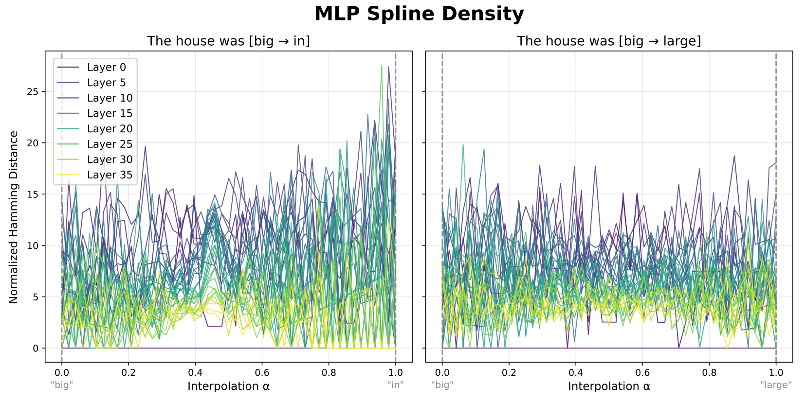
Shown above for each layer, this reveals a medium-sized jump in spline density at the same point in the interpolation where the plateau boundary occurs. This is fairly consistent across layers, and does not occur elsewhere or for the non-plateau case (right). This suggests that other findings from spline-based analyses may generalize to MLPs in LLMs.^[10][11]

More broadly, we think that investigating these and other connections are a promising route not just for understanding activation plateaus, but model representations and computations more broadly.

1. ^{^}

   Specifically, we use spherical interpolation to determine the directions of the interpolated points, and then rescale the interpolated points so that L2 magnitude of the vectors is linearly interpolated between the two endpoints. This prevents vector norms from becoming unusually small.

2. ^{^}

   We compute relative distance (d) as a function of the recorded outputs (x) and the two endpoints (A and B) using the following equation:
   d = ||x - A|| / (||x - A|| + ||x - B||)

3. ^{^}

   Given previous findings that plateau sharpness increases as a function of training time, a slight drop in plateau sharpness in the LayerNorm-free model may be explained by the fact that the initial LayerNorm removal substantially disrupted model behavior. They performed subsequent fine-tuning to restore the original model performance, but this may not have been enough to fully restore the original plateau sharpness, and further fine-tuning might result in even sharper plateaus.

4. ^{^}

   This doesn't preclude the possibility that LayerNorm is still important for plateaus in models which have it; it may just be that its role in producing plateaus is taken on by the FC layers of the MLP. Indeed, if we look at the norms of residual stream activations across the interpolation, we see a drop in magnitude around where the boundaries occur. If we then compute the Jacobian of the LayerNorm operation itself, the norm of the Jacobian is higher at these locations, just due to the fact that adding fixed-L2-magnitude perturbation to a vector changes the direction of the vector more if the vector itself is shorter.
   It's also worth keeping in mind that while this model does not have LayerNorm, it's fine-tuned from a model which does. A model trained from scratch without LayerNorm might learn mechanisms that do not involve this change in norm.

5. ^{^}

   This is expected, but not guaranteed; it's possible for two points to be far apart in activation space while still having the same relative distance from the two reference prompts.

6. ^{^}

   Taking the L2 norm of the whole Jacobian is a simple way to get an aggregate measure, but other metrics might be better. In particular, computing the directional Jacobian (e.g. by taking the product of the full Jacobian and the step direction) might better describe sensitivity along the direction(s) that activations actually vary along. Other possible metrics include pullback measures, other norms, or volume measures.

7. ^{^}

   As illustrated in the animation following this, 'sharpening' of the Jacobian spike is expected. While the interpolation steps start off evenly spaced at the interpolation layer, they quickly get pulled toward the two reference prompts and away from the plateau boundary. Consequently, only a few points in later layers still lie close to the boundary (where Jacobian norms are high), resulting in the apparent sharpening of the region of activation space where Jacobian norms are large.

8. ^{^}

   Here we assume, for simplicity in the illustration, that all layers have smooth, shallow curves like in the left column. In actuality, they may look different than this and vary more across layers, e.g. be higher in earlier layers.

9. ^{^}

   Future investigations of splines like these could be done with the OPT series of models, which do actually use ReLU in their MLPs.

10. ^{^}

    There are also promising intersections between splines and MLP Jacobians. For example, in ReLU MLPs, the input-output Jacobian is determined solely by active neurons (where the activations pass the ReLU threshold), and does not vary within a given polytope/spline code. In fact, if you're computing an aggregate metric over the Jacobian like the sum, you can precompute a scalar value per hidden neuron. You can then, for any spline code, compute the sum of the Jacobian by just summing these scalar values for the active neurons.

    This should allow you to compute which neurons need to be turned 'on' or 'off' to maximally increase or decrease the magnitude of the Jacobian. This could possibly be used to predict where plateaus and boundaries lie across input space. It could also be leveraged to determine which steering directions will push activations into new plateaus.

11. ^{^}

    See Interpreting Neural Networks through the Polytope Lens (Black et al., 2022) for other explorations along this vein.

Discuss