
Published on October 9, 2025 8:11 PM GMT
This is a summary of the project I undertook during SPAR, mentored by Ari Brill. I have recently had to prioritize other work, and found more questions than answers, as is often the case. I think a write-up will be useful both for coming back to this and interesting for the findings (and non-findings!) it presents.
Introduction
Real-world data is implicitly structured by the reality it represents, not just its surface-level format. AI systems can learn surface patterns, deeper structures, or a combination of both. Let's illustrate this with an example.
Take (the concept of) a dog, for instance. This dog can be represented by a picture, a GIF, a paragraph that describes it, a poem, or any other format that we can think of. Now, say we want to train an AI system to learn a function that involves said dog. This could be a function of the sort: f:Animal→Food, where f defines the animal´s favorite food. Now, in order to model f, the system[1] needs to represent the concept of a dog, and associate it to f(dog), which might be peanut butter. It might do so using surface level patterns (two ears, fluffy hair, four legs and paws) or by embedding the concept in a deeper way and truly representing the dog, which would intuitively mean having all similar dogs embedded close together in data space (which contains the remaining empirical degrees of freedom after accounting for invariances and symmetries).
The model described in [1] and [2] proposes a theoretical framework in which such deep structure naturally arises, with the assumptions described further below.
Building on the work of [3] and [4], we aim to advance fundamental scientific understanding of how AI systems internally represent the world. Our goal is to contribute to AI alignment by developing a model of data distributional geometric structure, which could provide an inductive bias for mechanistic interpretability.
In this work, we propose to empirically validate the learning model described in [1]. This relies on two key assumptions:
- Realistic target functions often reflect a mix of distinct behaviors rather than a single concept. We work with such context-dependent functions and model them as higher-order functions that produce task-specific first-order functions.We study general-purpose learning, where the system has no built-in knowledge of the data or task. We assume such a setting and treat the input format as statistically random, since it has no relation to the data's latent structure.
We use percolation theory [5] to study such a setting.
Theory
Some theoretical aspects relevant for context:
Below is a brief summary of key theoretical points; for a full treatment, please refer to [2].
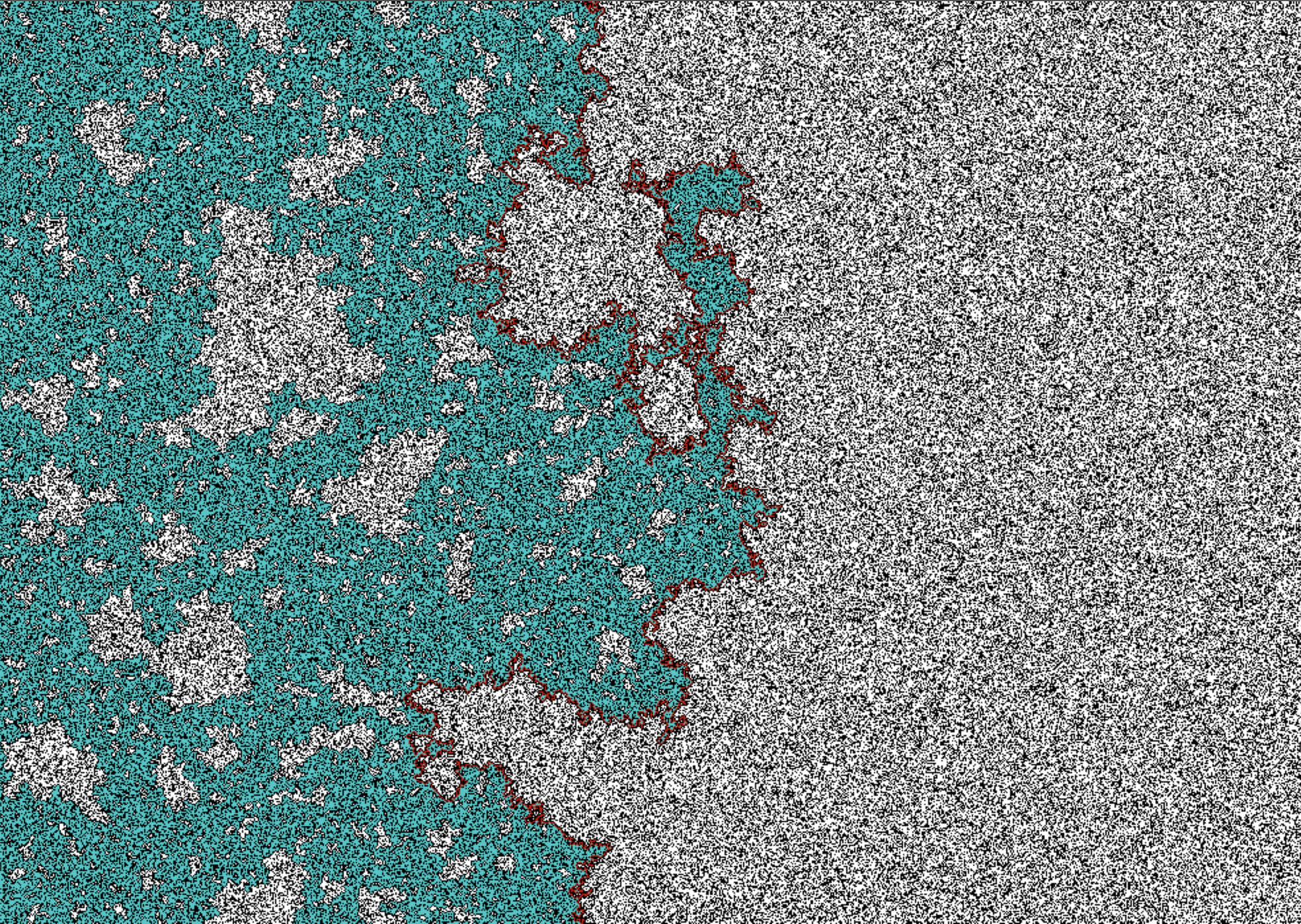
- Context-dependent target functions and general-purpose learning motivate a random lattice data distribution model, where elements are occupied at random with probability p, and we draw a bond xi∼xj if they share their context-dependent function, i.e. fxi(xi)=fxj(xi) and fxi(xj)=fxj(xj).The statistics and geometry of randomly occupied units on a lattice can be analyzed using percolation theory ([5]). Depending on the occupation probability p, the resulting data distribution either consists of a collection of distinct clusters that have a power-law size distribution, or is dominated by one infinite cluster, transitioning about a critical threshold pc. In this project, we for simplicity consider a data distribution consisting of a single percolation cluster at p=pc.We study percolation on a Bethe lattice as a tractable approximation of percolation on a hypercubic lattice of dimension d≥6 ([5], chapter 2.4).Percolation clusters in this setting have fractal dimension D=4.Manifold approximation scaling [4] predicts cD scaling for percolation clusters, with c depending on the ML method and activation function for a neural network.
Cluster embedding algorithm
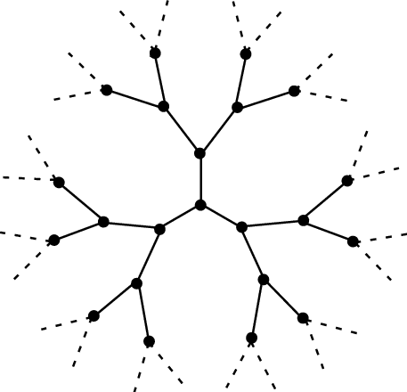
In order to test the scaling law predictions that emerge from the data model, we need to embed our representation of deep structure (a percolation cluster on the Bethe lattice) into Rd.
The criteria for the design of the embedding algorithm are: efficiency and correctness. By correctness, we mean an embedding of the lattice that is faithful to the lattice structure. This means that:
- It has fractal structure. This translates to the process being recursive, i.e. that at each node the process to generate the children is the same irrespective of the node considered.Child nodes should point in distinct directions that span the space while avoiding the backward direction toward their grandparent, since in the lattice such nodes are at discrete distance two. This preserves the local geometry of the lattice. For large d ( d≥6), random directions become nearly orthogonal, with distances between points on Sd−1 exceeding √d, so overlap between child directions is naturally avoided.Distance between consecutive nodes should be constant in data space Rd , modeling the lattice spacing in the percolation model. This will translate to us normalizing the random walk step to have an expected unit squared length.
Our base (naive) algorithm recursively takes a node with embedding coordinates x and generates a number of children k∼B(z=2d−1,p=12d−1), and embeds each of them in x+r, where r√d∼N(0,Id). This effectively meets 1, 2 and 3.
The problem with the naive process is that, for the results to be valid, the number of embedded nodes needs to be very large (in [2], the experiments go to ∼107 nodes) and this method is impractically memory inefficient. However, we can leverage the fractal structure of the embedding in the following process: generate an embedding of ^N nodes (large but small enough to fit in memory), then sample Nbranch nodes from it (thus reducing the memory usage by a factor of ^NNbranch); then further sample B−1 nodes from this dataset and generate B−1 embeddings in the same way, reducing them to a size of Nbranch, and displacing each of them to start at the corresponding sampled random node. This emulates the branching process having continued to a much larger dataset size. This is an approximate algorithm, because it assumes that all nodes are leaf nodes. This is a reasonable approximation, because for a large cluster about half of the nodes are leaf nodes. We therefore reach a dataset size of B×Nbranch which we can see as sampled from an embedding of size B×^N.
The final algorithm to embed a Bethe lattice efficiently into a d-dimensional space is shown below.
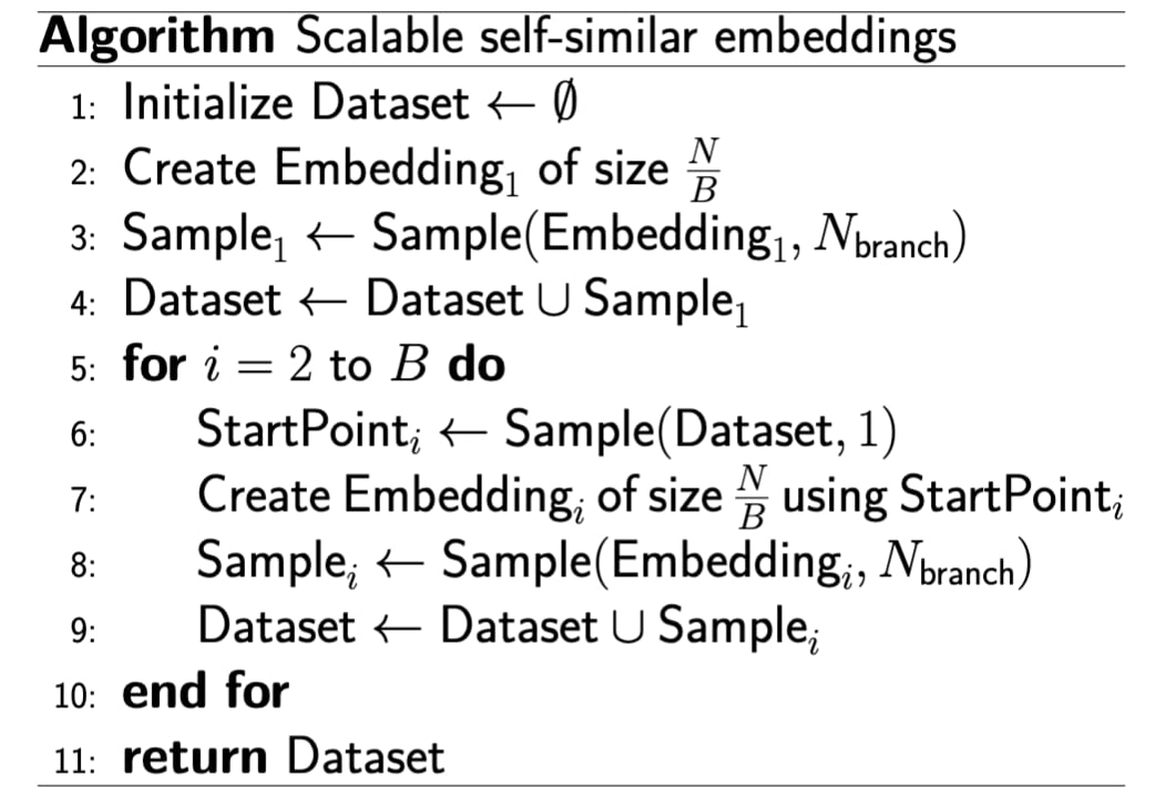
The resulting dataset has a total size of NbranchB sampled from a dataset of size N (setting ^N=NB), while only storing max(NbranchB,NB) coordinates at any time. This allows scaling to large N efficiently while preserving self-similarity.
First scaling experiments
We first performed scaling experiments on the embedded data using nonparametric ML models, extending the approach used in [2] where clusters were modeled as non-embedded graphs.The theoretically expected scaling law is given by [4], with the intrinsic dimension set to the embedded percolation cluster's fractal dimension D=4.
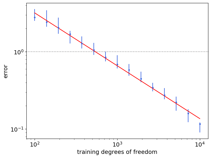
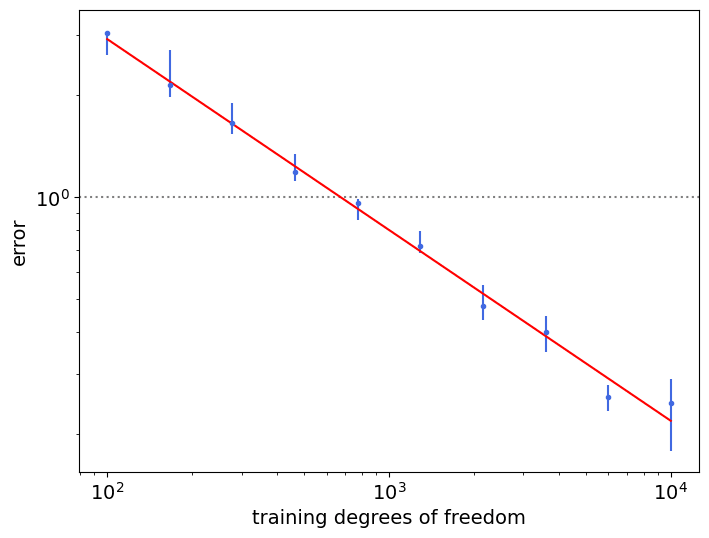
The plot below shows data scaling on on a single-cluster dataset fitted with 1-nearest neighbors (c=2), with one-dimensional regression labels obtained via a linear teacher function. Training degrees of freedom represent the number of points in our dataset.
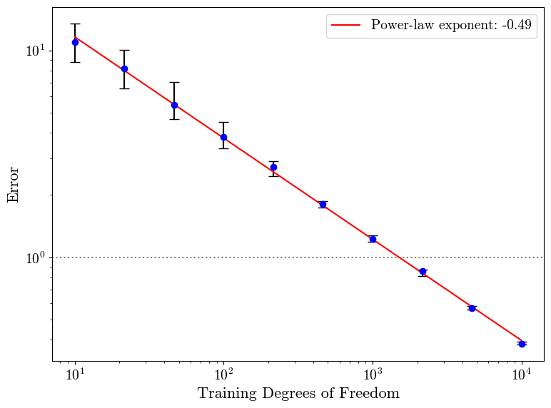
The results are independent of the embedding dimension d and branching factor B.
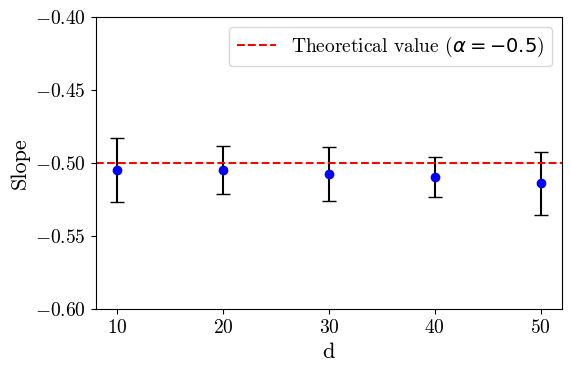
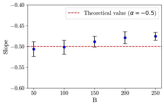
This provides evidence that the algorithm is doing what we want (as shown by the ablations on d and B) and that the scaling laws hold!
Extending scaling laws to neural networks
Next, we wanted to verify the scaling behavior of neural networks. This is harder, and often messier, as hyperparameter tuning and suboptimal training can confound the results. We generated random nonlinear functions following [4], using 2-layer ReLU-based networks with randomly generated weights and biases (w∼N(0,σ2)).
In general, when experimenting we ran a sweep to find the optimal hyperparameters for the student-teacher configuration and evaluated using the best-performing hyperparameters found. In what follows, we outline the main directions we explored in the hopes of understanding the scaling behavior that we observed.
Direction #1: Verifying the data dimension
The first scaling experiments proved unsuccessful. We were not seeing the expected power law scaling coefficients (slope in the log-log plots) even after extensive hyperparameter optimization.
Seeing this, we checked that the neural network could resolve the intrinsic dimension as expected (making the scaling behavior independent of d, the ambient dimension) and that the embedding algorithm indeed resulted in a structure of correct intrinsic dimension (i.e. the object our algorithm generates has intrinsic dimension D=4).
To check this, we used several intrinsic dimension estimation methods and found that while they do not agree on the measurements (which is expected, as estimating the intrinsic dimension of a dataset is an active research area) some converge to the expected number. However, the measurements were extremely noisy, and the method used in [4] did not converge to the expected number. In this method, the intrinsic dimension is estimated using the representation in the trained neural network's penultimate layer. It therefore assumes that the neural network has learned the function well and compresses the data well. Theoretically, the function learned needs to be generic to maintain the intrinsic dimension of the data (otherwise, a low-rank function could easily remove directions). For these reasons, we pivoted to studying the generated functions in more detail. Around this time, we decreased the dataset size in order to iterate faster. We also went back to the setup in [4] to see if we could reproduce and understand what was happening better.
Direction #2: Generating generic non-linear functions: random ReLU networks.
Using nonlinearity as a proxy for genericness, we conjectured and further observed that increasing the depth of the teacher network increased the non-linearity while keeping parameter count low[2]. This appeared to lead to the expected scaling behavior, both a data distribution consisting of a simple manifold [4] and for our fractal. However, the range in which we observed this scaling was very small, namely around [100,200], and we were quite skeptical of this result. Wanting to investigate this further, we moved to visualize some functions generated in this way.
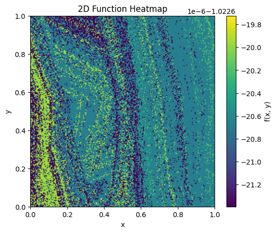
Visualizing some functions (and hence interpolating observations from two to higher dimensions), we observe that networks that have low width (~10) show a strange, grainy texture, and the range is sometimes small, as observed in an example below.
When looking at higher widths (~100), this problem disappears:
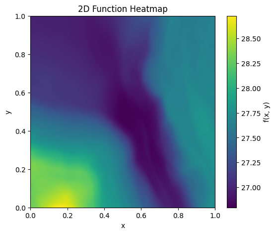
But wider teacher models did not change the scaling behavior.
In general, we observed that expected scaling behavior was correlated with high non-linearity[3], and implemented a naive vetting procedure to keep teacher networks with nonlinearity above a particular threshold, similar to [4]. Around this point, we started to wonder whether random ReLU teachers were a good way of constructing non-linear (and therefore generic, per our proxy) functions.
Direction #3: Generating generic functions: random Fourier networks.
To obtain smooth, non-linear functions, it occurred to us to try randomly generating coefficients from a subset of the Fourier basis. This was partially motivated by seeing that the plots show uneventful functions, with little variation across the studied domain, as can be seen in the images above.
To generate such a teacher, we generated a fixed number of basis elements with frequency ∈[−maxfreq,maxfreq] and added them together. We found that using max_freq = 1 induced expected scaling in the range [103,104], but not past it.
The problem with these teacher networks are twofold: they are slow to run inference, and convergence to optimal parameters requires both a lot of iterations and hyperparameter tuning. This is consistent with our findings: we chose them for their variations and genericness, and as such they are harder to optimize than simpler ReLU teachers that are not as generic and do not introduce that much variation.
Conclusion and further work
During this project, we started with the goal to validate a set of predictions based on [1] and ended up studying the particularities of neural scaling laws in neural networks. Overall, this project helped us gain insight into how a data distribution's intrinsic dimension and geometry, along with the genericness of the function imposed on it, may both play a role in producing neural scaling laws. It is also interesting (as non-findings often are) how difficult/challenging it was to reproduce neural scaling results, hinting at the volatility of the process and dependence on the elucidated factors.
I [Nathaniel] want to extend my heartfelt thanks to Ari for his mentorship and guidance during this project. Through our conversations and meetings, I feel as I have become a better scientist, truth-seeker and met a great person in the process.
References
[1] Brill, A. (2025). Representation Learning on a Random Lattice. arXiv [Cs.LG]. Retrieved from http://arxiv.org/abs/2504.20197
[2] Brill, A. (2024). Neural Scaling Laws Rooted in the Data Distribution. arXiv [Cs.LG]. Retrieved from http://arxiv.org/abs/2412.07942
[3] Michaud, E. J., Liu, Z., Girit, U., & Tegmark, M. (2024). The Quantization Model of Neural Scaling. arXiv [Cs.LG]. Retrieved from http://arxiv.org/abs/2303.13506
[4] Sharma, U., & Kaplan, J. (2022). Scaling Laws from the Data Manifold Dimension. Journal of Machine Learning Research, 23(9), 1–34. Retrieved from http://jmlr.org/papers/v23/20-1111.html
[5] Stauffer, D. & Aharony, A. Introduction to Percolation Theory.
Taylor & Francis, 1994.
- ^
We assume the system to be multimodal for the purpose of this example, though we could apply the same idea to a specific modality, say using different descriptions of the same dog.
- ^
This came from observing that Nparams≈depth∗(width)2 while Npieces≈(2∗width)depth, where Npieces is the number of linear pieces that a ReLU network has. Increasing depth is therefore the cheapest way (in parameter count) to increase the number of pieces, and hence the non-linearity.
- ^
Non linearity score is defined as in [2]. For a given teacher, take a random slice along each input coordinate axis (i.e. the values of the other coordinates are chosen uniformly at random from [−1/2,1/2)). Then perform linear regression on this slice and compute the R2 score, and take the mean of the scores across coordinate axes. A low score implies more non-linearity. Finally, repeat this procedure 200 times and compute the mean score of all the trials. This is the score for the teacher.
Discuss
